CODS example workflow¶

This juypter notebook is intended to give an introduction to the Combined Degradation and Soiling (CODS) algorithm workflow.

The calculations consist of several steps from the degradation_and_soiling_workflow. This is not meant as an introduction to the RdTools workflow in general, but we show how the CODS algorithm can be used in the context of the general RdTools workflow. The steps involved are:

Import and preliminary calculations
Normalize data using a performance metric
Filter data that creates bias
Aggregate and remove outliers
Run CODS on the aggregated data
Visualize the results of the CODS algorithm

This notebook works with public data from the the Desert Knowledge Australia Solar Centre. Please download the site data from Site 12, and unzip the csv file in the folder: ./rdtools/docs/

Note this example was run with data downloaded on Sept. 8th, 2020. An older version of the data gave different sensor-based results. If you have an older version of the data and are getting different results, please try redownloading the data.

http://dkasolarcentre.com.au/download?location=alice-springs

For more information about CODS, we refer to [1] and [2].

[1] Skomedal, Å. and Deceglie, M. G. IEEE J. of Photovoltaics, Sept. 2020 [2] Skomedal, Å., Deceglie, M. G., Haug, H., and Marstein, E. S., Proceedings of the 37th European Photovoltaic Solar Energy Conference and Exhibition, Sept. 2020

[1]:

from datetime import timedelta
import pandas as pd
import matplotlib.pyplot as plt
import numpy as np
import pvlib
import rdtools
from rdtools.soiling import CODSAnalysis
%matplotlib inline

/Users/mdecegli/opt/anaconda3/envs/cods_test/lib/python3.10/site-packages/rdtools/soiling.py:27: UserWarning: The soiling module is currently experimental. The API, results, and default behaviors may change in future releases (including MINOR and PATCH releases) as the code matures.
  warnings.warn(

[2]:

#Update the style of plots
import matplotlib
matplotlib.rcParams.update({'font.size': 12,
                           'figure.figsize': [4.5, 3],
                           'lines.markeredgewidth': 0,
                           'lines.markersize': 2
                           })
# Register time series plotting in pandas > 1.0
from pandas.plotting import register_matplotlib_converters
register_matplotlib_converters()

0: Import and preliminary calculations¶

[3]:

file_name = '84-Site_12-BP-Solar.csv'

df = pd.read_csv(file_name)
try:
    df.columns = [col.decode('utf-8') for col in df.columns]
except AttributeError:
    pass  # Python 3 strings are already unicode literals
df = df.rename(columns = {
    u'12 BP Solar - Active Power (kW)':'power',
    u'12 BP Solar - Wind Speed (m/s)': 'wind_speed',
    u'12 BP Solar - Weather Temperature Celsius (\xb0C)': 'Tamb',
    u'12 BP Solar - Global Horizontal Radiation (W/m\xb2)': 'ghi',
    u'12 BP Solar - Diffuse Horizontal Radiation (W/m\xb2)': 'dhi'
})

# Specify the Metadata
meta = {"latitude": -23.762028,
        "longitude": 133.874886,
        "timezone": 'Australia/North',
        "gamma_pdc": -0.005,
        "azimuth": 0,
        "tilt": 20,
        "power_dc_rated": 5100.0,
        "temp_model_params": pvlib.temperature.TEMPERATURE_MODEL_PARAMETERS['sapm']['open_rack_glass_polymer']}

df.index = pd.to_datetime(df.Timestamp)
# TZ is required for irradiance transposition
df.index = df.index.tz_localize(meta['timezone'], ambiguous = 'infer')

# Explicitly trim the dates so that runs of this example notebook
# are comparable when the sourec dataset has been downloaded at different times
df = df['2008-11-11':'2017-05-15']

# Chage power from kilowatts to watts
df['power'] = df.power * 1000.0

# There is some missing data, but we can infer the frequency from the first several data points
freq = pd.infer_freq(df.index[:10])

# Then set the frequency of the dataframe.
# It is reccomended not to up- or downsample at this step
# but rather to use interpolate to regularize the time series
# to it's dominant or underlying frequency. Interpolate is not
# generally recomended for downsampleing in this applicaiton.
df = rdtools.interpolate(df, freq, pd.to_timedelta('15 minutes'))

# Calculate energy yield in Wh
df['energy'] = rdtools.energy_from_power(df.power, max_timedelta=pd.to_timedelta('15 minutes'))

# Calculate POA irradiance from DHI, GHI inputs
loc = pvlib.location.Location(meta['latitude'], meta['longitude'], tz = meta['timezone'])
sun = loc.get_solarposition(df.index)

# calculate the POA irradiance
sky = pvlib.irradiance.isotropic(meta['tilt'], df.dhi)
df['dni'] = (df.ghi - df.dhi)/np.cos(np.deg2rad(sun.zenith))
beam = pvlib.irradiance.beam_component(meta['tilt'], meta['azimuth'], sun.zenith, sun.azimuth, df.dni)
df['poa'] = beam + sky

# Calculate cell temperature
df['Tcell'] = pvlib.temperature.sapm_cell(df.poa, df.Tamb, df.wind_speed, **meta['temp_model_params'])

1: Normalize¶

[4]:

# Specify the keywords for the pvwatts model
pvwatts_kws = {"poa_global" : df.poa,
              "power_dc_rated" : meta['power_dc_rated'],
              "temperature_cell" : df.Tcell,
              "poa_global_ref" : 1000,
              "temperature_cell_ref": 25,
              "gamma_pdc" : meta['gamma_pdc']}

# Calculate the normaliztion, the function also returns the relevant insolation for
# each point in the normalized PV energy timeseries
normalized, insolation = rdtools.normalize_with_pvwatts(df.energy, pvwatts_kws)

df['normalized'] = normalized
df['insolation'] = insolation

2: Filter¶

[5]:

# Calculate a collection of boolean masks that can be used
# to filter the time series
normalized_mask = rdtools.normalized_filter(df['normalized'])
poa_mask = rdtools.poa_filter(df['poa'])
tcell_mask = rdtools.tcell_filter(df['Tcell'])
clip_mask = rdtools.clip_filter(df['power'])

# filter the time series and keep only the columns needed for the
# remaining steps
filtered = df[normalized_mask & poa_mask & tcell_mask & clip_mask]
filtered = filtered[['insolation', 'normalized']]

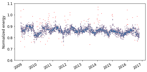
3: Aggregate and remove outliers¶

[6]:

# Calculate the daily normalized energy
daily = rdtools.aggregation_insol(filtered.normalized, filtered.insolation, frequency = 'D')

# Plot unfiltered data
fig, ax = plt.subplots(figsize=(8, 4))
ax.plot(daily.index, daily, 'o', color='r', alpha=.7)
ax.set_ylim(0.6, 1.1)
fig.autofmt_xdate()
ax.set_ylabel('Normalized energy');

# The CODS algorithm typically performs better if outliers are removed,
# for instance in this manner
rolling_median = daily.rolling(15, 1, center=True).median()
noise = (daily - rolling_median).abs()
Q3, Q1 = noise.quantile(.75), noise.quantile(.25)
outliers = noise > Q3 + 3 * (Q3 - Q1)
daily[outliers] = np.nan

# Plot filtered data
ax.plot(daily.index, daily, 'o', alpha=.7)

[6]:

[<matplotlib.lines.Line2D at 0x7f8284598100>]

../_images/examples_cods_example_10_1.png

4: Run CODS¶

CODS can be run in two ways - either by setting up an instance of rdtools.soiling.CODSAnalysis and running the method run_bootstrap, or by directly running rdtools.soiling.soiling_cods. Here we will show how to do the first option, as this makes more information available, and since the second option is more straightforward. We start by setting up an instance of rdtools.soiling.CODSAnalysis:

[7]:

CODS = CODSAnalysis(daily)

We continue to run run_bootstrap. The parameter reps decides how many repetitions of the bootstrapping procedure should be performed. reps needs to be a multiple of 16, and the minimum is 16. However, to give real confidence intervals, we recommend running it with 512 repetitions. In this case we use 16 to to avoid overly much time use. The parameter verbose decides whether to output information about the process during the calculation.

[8]:

results_df, degradation, soiling_loss = CODS.run_bootstrap(reps=16, verbose=True)

Initially fitting 16 models
# 16 | Used: 1.8 min | Left: 0.0 min | Progress: [----------------------------->] 100 %
            order    dt        pt     ff      RMSE     SR==1   weights  \
0   (SR, SC, Rd)  0.25  0.666667   True  0.016755  0.137289  0.064653
1   (SR, SC, Rd)  0.25  0.666667  False  0.016978  0.155571  0.062793
2   (SR, SC, Rd)  0.25  1.500000   True  0.016847  0.166954  0.062662
3   (SR, SC, Rd)  0.25  1.500000  False  0.016872  0.166954  0.062572
4   (SR, SC, Rd)  0.75  0.666667   True  0.016895  0.143153  0.063785
5   (SR, SC, Rd)  0.75  0.666667  False  0.017056  0.143153  0.063185
6   (SR, SC, Rd)  0.75  1.500000   True  0.016964  0.167299  0.062213
7   (SR, SC, Rd)  0.75  1.500000  False  0.017116  0.199034  0.060028
8   (SC, SR, Rd)  0.25  0.666667   True  0.016884  0.153501  0.063254
9   (SC, SR, Rd)  0.25  0.666667  False  0.016964  0.161090  0.062548
10  (SC, SR, Rd)  0.25  1.500000   True  0.016836  0.166954  0.062706
11  (SC, SR, Rd)  0.25  1.500000  False  0.016885  0.175578  0.062064
12  (SC, SR, Rd)  0.75  0.666667   True  0.016906  0.143843  0.063706
13  (SC, SR, Rd)  0.75  0.666667  False  0.017072  0.153501  0.062559
14  (SC, SR, Rd)  0.75  1.500000   True  0.016984  0.172473  0.061867
15  (SC, SR, Rd)  0.75  1.500000  False  0.017168  0.208003  0.059404

    small_soiling_signal
0                  False
1                  False
2                  False
3                  False
4                  False
5                  False
6                  False
7                  False
8                  False
9                  False
10                 False
11                 False
12                 False
13                 False
14                 False
15                 False

Bootstrapping for uncertainty analysis (16 realizations):
# 16 | Used: 0.5 min | Left: 0.0 min | Progress: [----------------------------->] 100 %
Final RMSE: 0.01722

Another alternative, if you don’t need confidence intervals, is to run the iterative_signal_decomposition-method. It gives you all the different component estimates, but it does not use time on doing bootstrapping, so it is much faster than the run_bootstrap-method:

[9]:

df_out, CODS_results_dict = \
    CODS.iterative_signal_decomposition()
df_out.head()

[9]:

	soiling_ratio	soiling_rates	cleaning_events	seasonal_component	degradation_trend	total_model	residuals
2008-11-14 00:00:00+09:30	1.0	-0.005374	False	0.993214	1.000000	0.891288	0.903519
2008-11-15 00:00:00+09:30	1.0	0.000000	False	0.993258	0.999985	0.891314	0.937192
2008-11-16 00:00:00+09:30	1.0	0.000000	False	0.993304	0.999969	0.891342	NaN
2008-11-17 00:00:00+09:30	1.0	0.000000	False	0.993353	0.999954	0.891372	NaN
2008-11-18 00:00:00+09:30	1.0	0.000000	False	0.993404	0.999938	0.891404	0.912726

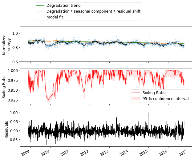
5: Visualize the results¶

[10]:

# The average soiling loss over the period with 95 % confidence intervals
# can be accessed through the soiling_loss attribute of CODS
soiling_loss = CODS.soiling_loss
print('Avg. Soiling loss {:.3f} ({:.3f}, {:.3f}) (%)'.format(soiling_loss[0], soiling_loss[1], soiling_loss[2]))

# The estimated degradatio rate over the period with 95 % confidence intervals
# can be accessed through the degradation attribute of CODS
degradation = CODS.degradation
print('Degradation rate {:.3f} ({:.3f}, {:.3f}) (%)'.format(degradation[0], degradation[1], degradation[2]))

Avg. Soiling loss 1.854 (1.436, 2.300) (%)
Degradation rate -0.555 (-0.647, -0.474) (%)

[11]:

# The dataframe containing the time series of the different component fits
# can be accessed through CODS.result_df
result_df = CODS.result_df

# Let us plot the time series of the results
# First: daily normalized energy along with the total model fit and degradation trend
fig, (ax1, ax2, ax3) = plt.subplots(3, 1, figsize=(10, 8))
ax1.plot(daily.index, daily, 'o', alpha = 0.3)
ax1.plot(result_df.index, result_df.degradation_trend * CODS.residual_shift, color='g', linewidth=1,
         label='Degradation trend')
ax1.plot(result_df.index, result_df.degradation_trend * result_df.seasonal_component * CODS.residual_shift,
         color='C1', linewidth=1, label='Degradation * seasonal component * residual shift')
ax1.plot(result_df.index, result_df.total_model, color='k', linewidth=1,
         label='model fit')
ax1.set_ylim(0.6, 1.1)
ax1.set_ylabel('Normalized\nenergy')
ax1.legend(bbox_to_anchor=(0.075, 1.1))

# Second: soiling ratio with 95 % confidence intervals
ax2.plot(result_df.index, result_df.soiling_ratio, color='r', linewidth=1,
         label='Soiling Ratio')
ax2.fill_between(result_df.index, result_df.SR_low, result_df.SR_high,
                 color='r', alpha=.1, label='95 % confidence interval')
ax2.set_ylabel('Soiling Ratio')
ax2.legend()

# Third: The residuals
ax3.plot(result_df.index, result_df.residuals, color='k', linewidth=1)
ax3.set_ylabel('Residuals');

fig.autofmt_xdate()

../_images/examples_cods_example_19_0.png

[12]:

result_df

[12]:

	soiling_ratio	soiling_rates	cleaning_events	seasonal_component	degradation_trend	total_model	residuals	SR_low	SR_high	rates_low	rates_high	bt_soiling_ratio	bt_soiling_rates	seasonal_low	seasonal_high	model_low	model_high
2008-11-14 00:00:00+09:30	1.000000	-0.005341	0.000000	0.990558	1.000000	0.885361	0.905941	0.994225	1.000000	-0.005210	-0.000645	0.870846	-0.002532	0.987448	0.993431	0.889557	0.896195
2008-11-15 00:00:00+09:30	1.000000	0.000000	0.000000	0.990636	0.999985	0.885417	0.939673	0.994684	1.000000	0.000000	0.000000	0.870787	-0.000067	0.987471	0.993522	0.889546	0.896180
2008-11-16 00:00:00+09:30	1.000000	0.000000	0.000000	0.990716	0.999970	0.885475	NaN	0.990896	1.000000	-0.000450	0.000000	0.927635	-0.000412	0.987498	0.993616	0.888679	0.895974
2008-11-17 00:00:00+09:30	1.000000	0.000000	0.000000	0.990798	0.999954	0.885535	NaN	0.990092	1.000000	-0.000900	0.000000	0.927152	-0.000734	0.987528	0.993710	0.886391	0.895959
2008-11-18 00:00:00+09:30	1.000000	0.000000	0.000000	0.990883	0.999939	0.885597	0.915047	0.988270	1.000000	-0.004436	0.000000	0.995945	-0.001552	0.987563	0.993807	0.886462	0.895439
...	...	...	...	...	...	...	...	...	...	...	...	...	...	...	...	...	...
2016-10-17 00:00:00+09:30	0.969627	-0.000790	0.121848	0.989440	0.956025	0.819793	0.872090	0.962384	0.976346	-0.001528	-0.000530	0.969440	-0.000962	0.987038	0.992228	0.822338	0.836088
2016-10-18 00:00:00+09:30	0.968839	-0.000788	0.069925	0.989441	0.956010	0.819114	0.890061	0.960955	0.974488	-0.001528	-0.000523	0.968502	-0.000961	0.987123	0.992219	0.821738	0.836060
2016-10-19 00:00:00+09:30	0.968051	-0.000787	0.000000	0.989446	0.955995	0.818439	0.906098	0.959526	0.972967	-0.001528	-0.000522	0.967544	-0.000960	0.987212	0.992213	0.821140	0.836032
2016-10-20 00:00:00+09:30	0.967265	-0.000786	0.000000	0.989454	0.955980	0.817768	0.907413	0.958098	0.971972	-0.001528	-0.000522	0.966587	-0.000960	0.987249	0.992210	0.820543	0.836005
2016-10-21 00:00:00+09:30	0.973523	-0.000422	0.000000	0.989464	0.955965	0.823054	0.949943	0.957160	0.971610	-0.001501	-0.000484	0.965998	-0.000939	0.987286	0.992209	0.820396	0.836119

2899 rows × 17 columns